|
|


Hi, I'm John Nevins and I teach Biology and Physics at Crandon High
School. Our school has about 1200 in grades K-12 in a community of about
2000. Crandon is located in northcentral Wisconsin about three hours
north of Madison. This area is generally regarded as the north woods of
Wisconsin and my home is in Rhinelander.
I live on the Moen Lake chain with my wife Dorene, daughter Amanda 9, son
Michael 6, two dogs Taz and Tucker, a garter snake Tito, four fire-bellied
newts, and several fish. My family and I enjoy outdoor sports and
activities which include camping, canoeing, hunting and biking. Amanda
and Michael play soccer, baseball and are going to start waterskiing this
summer.
Our home is located in a region that was glaciated several times and we
have some interesting drainage patterns and landforms as a result. For
example, water from our lake travels down the Mississippi River drainage
system but the water at the Crandon school travels to Lake Michigan. This
means that I cross the Midcontinental Divide each day on the way to work.
This sounds impressive but you would probably not notice the divide when
you cross it as the hill is not any different than several others that you
would cross between Crandon and Rhinelander.
This was my second trip to Alaska but it was my first chance to
travel north of Fairbanks. The last time I was in Alaska was while I was
in college when I was looking for a summer job. On that trip I worked on
Kodiak Island at a store. I was really excited about my trip last summer as I
worked on a research project in the Kuparuk River basin. I had
always wanted to work with a research project in actual data collection
and I couldn't wait to start.
Kuparuk River field region.
The research project I'm involved with is titled "Active layer/landscape interactions: a
retrospective and contemporary approach in arctic Alaska." The project is headed by Dr. Fritz Nelson
of the Department of Geography, University of Delaware. It addresses several of the central questions of
the ARCSS/LAII (Arctic System Science/Land-Atmosphere-Ice Interactions) Flux Study, a multi-
project undertaking examining the flux of greenhouse gases from the tundra to the atmosphere
and hydrosphere in northern Alaska. The active layer is the layer of seasonally thawed and frozen ground
between the atmosphere and the permafrost in cold regions. If global warming affects the Arctic as
severely as climatic models predict, the thickness of the active layer may increase, which could lead to
release of carbon dioxide and methane currently stored in the upper permafrost. Release of large
quantities of these gases could bring about further climatic changes.
Our project is attempting to map the thickness of the active layer in the Kuparuk River basin
of north-central Alaska to provide a detailed description of the soils of this region, and to provide an
estimate of the organic carbon contained in the near-surface soils. Detailed maps of the active layer
have not been previously constructed for a region as large as the Kuparuk basin map area (28,000 square
kilometers). The material that follows introduces the people who parcticipated in the field work in
Alaska and outlines the methods that we used to map the Kuparuk active layer.
I. An introduction to some of the people who worked with John on the North Slope.
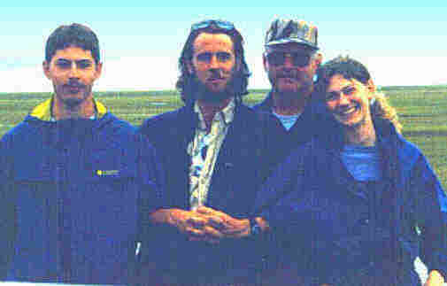 Jeremy, Jerry, John and Anna before heading out to probe the 1km x 1km site at West Dock Jeremy, Jerry, John and Anna before heading out to probe the 1km x 1km site at West Dock
Jeremy Harris is one of the high school student parcticipants in the Teachers Experiencing the
Arctic/Antarctic. He is a Senior at Abingdon High School, in Abingdon, Virginia. Jerry Mueller
completed his Masters degree in Geography at the State University of New York at Albany in May. He is currently traveling and doing art work. John Nevins was introduced earlier. Anna Klene is currently working on her M.A. in Geography at Albany. Her thesis examines the energy balance at the interface between the atmosphere and the ground in the Kuparuk River Basin.
Not shown in the photo are Nickolai Shiklomanov, a doctoral student at the University of
Delaware and Fritz Nelson, a professor at Delaware. Until September of 1997 both Nickolai and Fritz
worked at SUNY-Albany. Their current projects are developing different models to simulate active layer development that can be incorporated in general circulation models, and working on climate-change scenarios in the northern latitudes. Both were involved in the 1997 field activities and in laboratory work before and after the field season. Mike Walegur also did field work in Alaska this summer. His thesis focuses on another project, concerned with the relationship between temperature, elevation, and latitude in the Appalachian Mountains.
Other individuals involved with the active layer field work included Ken Hinkel, Wendy Eisner,
Sam Outcalt, and Laura Miller (all of the University of Cincinnati), Jim Bockheim (University of Wisconsin), and Lynn Everett (Ohio State University).
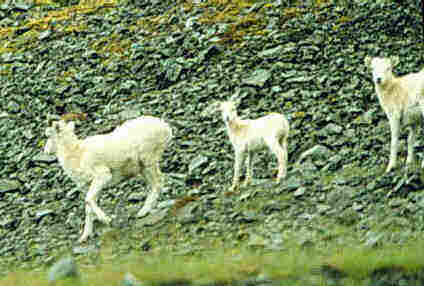
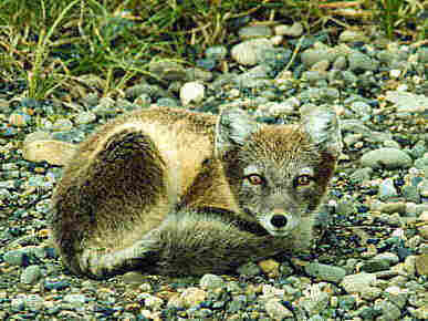
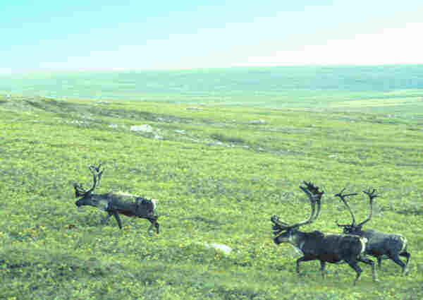 A few of the other parcticipants... the Animals.
Several of other individuals took part in the field activities in Alaska, including the sheep, fox and caribou seen here. We also encountered grizzly bears, musk oxen, eagles, owls, and lots of ground squirrels and mosquitoes!
II. Field Activities
The Kuparuk River basin (watershed) occupies an area of 9200 square kilometers in north
central Alaska. The terrain in the region ranges from very gently sloping, lake-dotted tundra in the
northern part of the study area to the rugged glacier-carved peaks of the Brooks Range in the south.
The intermediate portion of the map area is occupied by the foothills of the Brooks Range. The shaded
relief map immediately below gives a good impression of how varied the topography is in the study area.
We conducted detailed field studies at the locations shown by diamond and square symbols on the map.
The diamonds represent the 1 hectare (100 x 100 meter) "Flux Study Plots," which were used by several of
the Flux Study projects for determinating of methane and carbon dioxide fluxes, soil properties, active
layer thickness, vegetation composition, energy balance, and permafrost temperature. Each of the Flux
Study plots incorporates a distinct vegetation/soil association. The squares represent the locations of
the 1 square kilometer (1000 x 1000 meter) "ARCSS Grids," which are precisely surveyed arrays of
markers spaced at 100 meter horizontal intervals. These grids are also used by several projects, for a
variety of purposes. The ARCSS grids provide an integrated picture of local vegetation, soil,
and topographic characteristics. We worked at most of the Flux Study Plots and ARCSS Grids during
August of 1997.
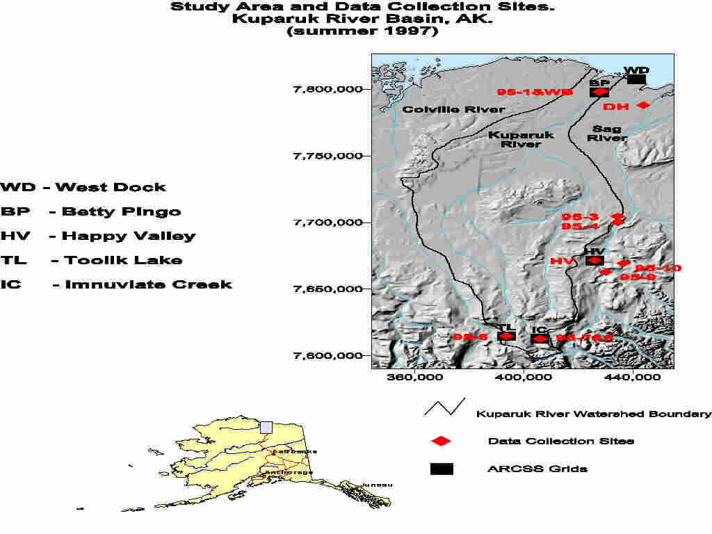 A map of the Kuparuk River Basin A map of the Kuparuk River Basin
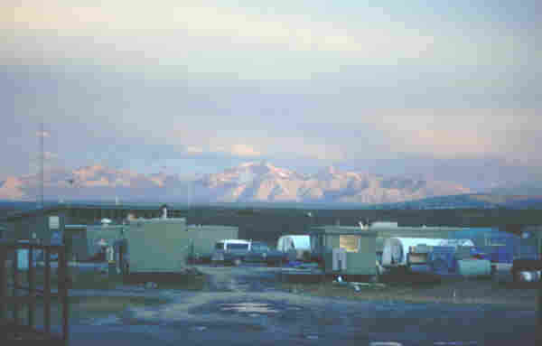 Toolik camp at dusk (1 AM). Toolik camp at dusk (1 AM).
Much of our work centered around the University of Alaska's Toolik Lake Field Station,
which receives support from the National Science Foundation. The Toolik Lake Station can
accomodate up to 130 scientists and serves as the base for helicopter operations in support of NSF-
funded science projects. The Kuparuk River region was an inaccessible wilderness until about 20 years
ago, when the Prudhoe Bay Oilfield and Trans-Alaska Pipeline System (TAPS) were developed.
TAPS and its service road (now known as the Dalton Highway) follow a north-south route through
the eastern part of our map area. We worked extensively at sites within the Prudhoe Bay Oilfield and
along the TAPS corridor (see photos). We also used a helicopter to make observations at
inaccessible sites located far from the pipeline corridor.
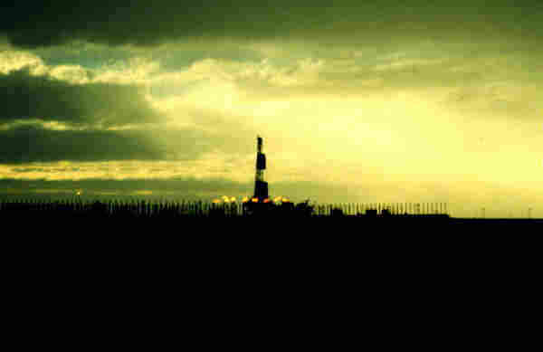
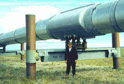
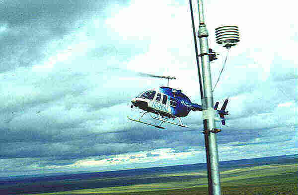 An oil rig at Prudhoe Bay, John by the Pipeline, and the helicopter taking off behind one of the masts with radiation shield and temperature logger.
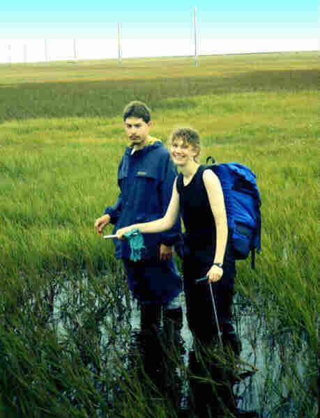
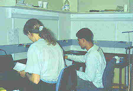 Our observation program was a mix of modern technology and old-fashioned manual
observation techniques. At each of the Flux Study Sites we used steel probes to determine the distance
between the surface and the bottom of the active layer (photo left). These data sets were
transcribed from our field notebooks into computer-readable format each night in the laboratory at the
Toolik base camp (photo right). Probing is done at each of the Flux Study plots and ARCSS grids at least three times during the summer, so that we can compute a rate of thaw for each of the different land-cover types. See Jeremy and Anna hard at work!
Our observation program was a mix of modern technology and old-fashioned manual
observation techniques. At each of the Flux Study Sites we used steel probes to determine the distance
between the surface and the bottom of the active layer (photo left). These data sets were
transcribed from our field notebooks into computer-readable format each night in the laboratory at the
Toolik base camp (photo right). Probing is done at each of the Flux Study plots and ARCSS grids at least three times during the summer, so that we can compute a rate of thaw for each of the different land-cover types. See Jeremy and Anna hard at work!
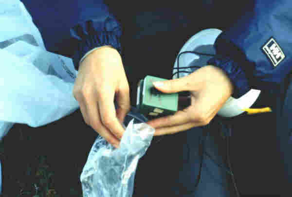  We also have several miniature data loggers collecting temperature records at each of the plots (see photos left and right). By summing mean daily temperatures above zero degrees Celsius, we obtain the "degree days of thaw" for the warm season. The degree-day sum is a measure of cumulative summer
warmth, and is used in many kinds of research and applied work to predict the depth of thaw in soils.
We used a relatively simple approximation, known as the "Stefan solution," to compute an estimate of the
thickness of the thawed layer. We also have several miniature data loggers collecting temperature records at each of the plots (see photos left and right). By summing mean daily temperatures above zero degrees Celsius, we obtain the "degree days of thaw" for the warm season. The degree-day sum is a measure of cumulative summer
warmth, and is used in many kinds of research and applied work to predict the depth of thaw in soils.
We used a relatively simple approximation, known as the "Stefan solution," to compute an estimate of the
thickness of the thawed layer.
The diagram below left shows the relation between geographic position (latitude) and the
degree-day totals for 1997 in the Kuparuk region. The degree-day totals increase steadily from north
(on the right of the diagram) to the south. The effects of elevation on the degree-day totals have been
filtered out of the relationship shown in this diagram. The graph below right shows the relation between
the degree-day sums and the depth of thaw for two of the Flux Study plots. Even though the rate of
thaw is very different in the five land-cover types shown, the relation between the thickness of the
thawed layer and the square root of the degree-day total is nearly linear, and is characteristic of thaw
progression in most places.
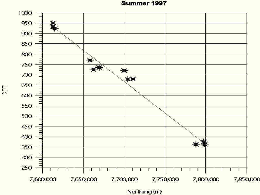
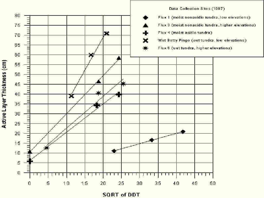 Latitude vs. Degree Days of Thaw, left, and Square Root of Degree Days vs. Active-Layer Thickness right.
Click the right mouse button on top of the images to enlarge them and examine the graphs.
Latitude vs. Degree Days of Thaw, left, and Square Root of Degree Days vs. Active-Layer Thickness right.
Click the right mouse button on top of the images to enlarge them and examine the graphs.
III. Analysis
After our return from Alaska, the data sets collected in the field required extensive
preprocessing to get them into a format to analyze and display the geographic relationships between
variables. We used geographic information systems (GIS) technology to create a series of digital
maps representing several important variables that are part of our procedures for extrapolating active-layer
thickness over the entire Kuparuk basin. The diagram below gives a schematic representation of
the steps that go into turning our field-based observations into maps. We had a short reunion in
Albany in mid-November and completed the series of maps represented in the diagram below.
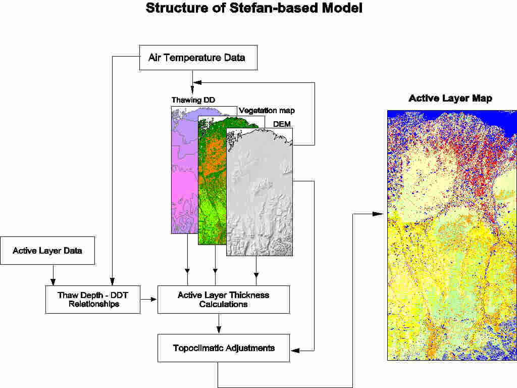 An illustration of the model for calculating Active-Layer Thickness
The intermediate steps include adjusting degree-day sums to the appropriate elevation at each
of the approximately 292,000 nodes on the Kuparuk digital terrain map, and creating a separate map of
the degree-day totals. We then used a digital land-cover map, created from satellite imagery by Dr.
Skip Walker (University of Colorado), to determine which of the Stefan equations to use at
parcticular points on the map. The appropriate Stefan relation allows us to compute an estimate of
the thickness of the active layer at each node. The result is shown below as a map of active-layer
thickness for mid-August of 1997. Comparing this map with similar ones that were computed for 1995
and 1996, we found that the active layer was slightly thinner in the northern part of the study area this
year. The primary reason for this is the cooler temperatures that prevailed near the coast in 1997.
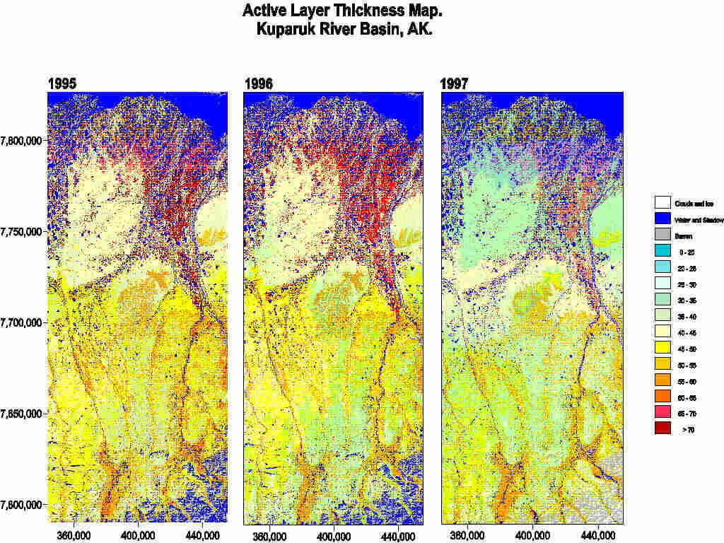
The resulting Active-layer Thickness Maps from the last 3 summers
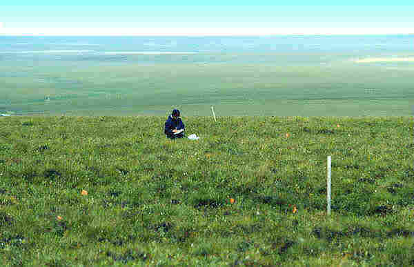
During the second half of August, we traveled by small, fixed-wing aircraft (photo below) to
the communities of Barrow and Atqasuk, which are located about 150 km west of the Kuparuk
study area. In Barrow, we continued our work on investigating the relationship between the active
layer and climate, and also collected data that will be used to construct a map of the carbon content of
soils in the Barrow Environmental Observatory. At Atqasuk we made a series of baseline
measurements on the active layer and climate. We also helped out with some work for the International
Tundra Experiment (ITEX), a project investigating the possible effects of climatic warming on tundra
vegetation. The ITEX program at Barrow is run by Dr. Pat Webber of Michigan State University, with
support from NSF's Office of Polar Programs. The Barrow and Atqasuk areas will continue to be
investigated intensively over the next several years by several research programs funded by the
U.S. Environmental Protection Agency, the National Oceanic and Atmospheric Administration, and
the National Science Foundation.
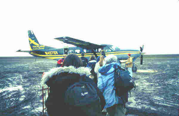
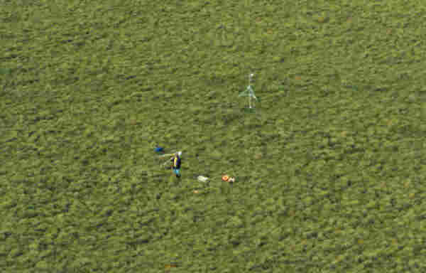 Boarding the plane in Barrow, and a low, oblique aerial view of one of the flux sites, with researcher, mast, and other equipment.
For more information on this research, see Nelson, et al., 1997, Estimating Active-Layer Thickness over a Large Region: Kuparuk River Basin, Alaska, Arctic and Alpine Research, vol. 29, no. 4, pp. 367-378.
IV. A Note from John...
In the following sections you will find a journal of my field experiences in the Arctic. The journal entries were written at the conclusion of each day in the field. I hope that some of the wonder of the experience will transfer to the reader. As you can see in the photos, we worked in a large variety of landforms and traveled rather large distances to accomplish the data collection for this study. I have seldom had the opportunity to work with such an outstanding group of individuals, and at the same time enjoyed working so hard. Before this journey, I would have been surprised at how far we walked in the typical day and how much data we recorded in that time. This has been an experience I would gladly repeat.
Polar Classroom Activities:
Global Change in the Arctic Tundra?
Overview
- Introduction to Field Data Collection
Part 1: Counting the Uncountable
Part
2: Data Collection and Analysis
August 1997
July 1997
| Su |
Mo |
Tu |
We |
Th |
Fr |
Sa |
| -- |
-- |
1 |
2 |
3 |
4 |
5 |
| 6 |
7 |
8 |
9 |
10 |
11 |
12 |
| 13 |
14 |
15 |
16 |
17 |
18 |
19 |
| 20 |
21 |
22 |
23 |
24 |
25 |
26 |
| 27 |
28 |
29 |
30 |
31 |
-- |
-- |
Return to top of page
|