
|

I.The Project: Active Layer /
Landscape Interactions in Arctic Alaska: a Retrospective and Contemporary
Approach.
The active layer study is focused on
gathering data about the near-surface permafrost and the layer of seasonally
frozen ground ("active layer") that is above it. With climate changes,
the active layer could drastically change in thickness. This means that
there is more (if the climate warms) or less (if the climate cools) material
that can release greenhouse gases to our atmosphere. This release may influence
existing hydrological patterns and also impact humans in settled areas
of the North Slope of Alaska. This project is part of a larger modeling
project that addresses the changes in geographic factors through time that
affect the active layer. We will be taking intensive measurements of temperature
and thaw depth, as well as others, over a large area centered primarily
along the Dalton Highway. II. People: Some of the people Don worked with this summer.
Javier Lopez was one of the student parcticipants in NSF's Young Scholars Program who accompany some of the TEA projects. He is a senior at River Ridge High in Spring Hill, Florida. His daily journal and photos, along with the other students' journals, are available on the web at http://www.arcus.org/TEA_StudentWebSite/journals.htm. Don Rogers was introduced earlier. Anna Klene is a graduate student completing her M.A. at the State University of New York at Albany, while beginning a Ph.D. at the University of Delaware. Not shown in the photo are Fritz Nelson and Nikolay (Kolia) Shiklomanov. Fritz Nelson, a professor at the University of Delaware, has been doing research in northern Alaska since the early 1980s. His specialty is climatic geomorphology, which means the study of the interactions between landscapes and climate. Kolia Shiklomanov is a doctoral student at UDel. He has developed several computer models to map and predict active-layer thickness in the Kuparuk River Basin and is now working on a model that can be used for larger areas. We were lucky to be part of a great research team
in 1998: Claire Gomersall, Wendy Eisner, Ken Hinkel,
Laura
Miller, and Sam Outcalt are all associated with the University
of Cincinnati, while Jim Bockheim and Jim O'Brien are at
the University of Wisconsin, and Ron Paetzold is with the Natural
Resources Conservation Service.
 Don worked in and around the Kuparuk River Basin. He was based out of Toolik Lake Field Station, Prudhoe Bay, and the Naval Arctic Research Laboratory at Ilisagvik College in Barrow. Northern Alaska encompasses over 200,000 square miles.&nbs\ p; It is comprised of three primary regions: the Coastal Plain, Foothills, and Brooks Range (Wahrhaftig, 1965). Don traveled through all three as part of his work. There are two groups of study sites at which we collected data in 1998. The "Flux Study" involves a transect of 10 square plots (100m x 100m) that parallel the Dalton Highway from the coast of the Arctic Ocean for 150 miles southward to Toolik Lake at the base of the Brooks Range. Groups of scientists have investigated the vegetation, soil properties, energy balance, permafrost, and carbon dioxide and methane fluxes at each plot. Another set of seven study sites are known as the "ARCSS Grids." These sites are much larger (1000m x 1000m) but have been precisely surveyed and staked at 100m intervals for long-term scientific studies. Vegetation, soils, and landforms are represented at a coarser spatial scale by these grids.
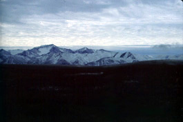
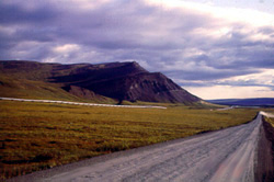
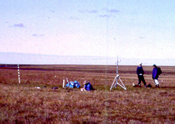
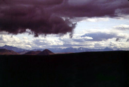
The three physiographic provinces of Northern Alaska (Wahrhaftig, 1965): the Brooks Range (near Atigun Pass), the Foothills (Slope Mt., notice the oil pipeline and part of the Dalton Highway), and the Coastal Plain (Atqasuk ARCSS grid, note L to R: survey marker, data logger and Ken Hinkel on ground, air temperature mast, Don Rogers and Fritz Nelson, photo by Anna Klene). We gathered two primary types of data: temperature and active-layer thickness. The active layer is the upper portion of the soil which freezes and thaws on an annual basis. Beneath the active layer is permafrost or "permanently frozen ground." Permafrost can be close to the surface (>30cm) or quite deep, and it's thickness can range from a few meters to more than a thousand.
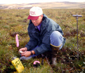
Left: Don unwrapping a datalogger; notice the probe on the right side of the photo. Below right: A close-up of a piece of PVC pipe, two dataloggers, plastic bags, and the always essential duct tape.
Top to bottom: North Slope Borough seal, Don and Anna enter data in one of Toolik's dry labs, and Javier standing next to polygons eroding into the Sagavanirktok River near Deadhorse (photo by Anna Klene).
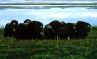
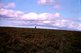
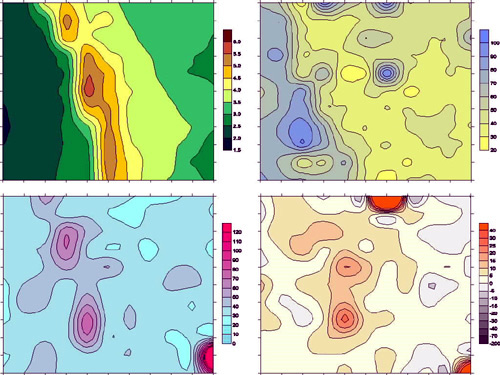
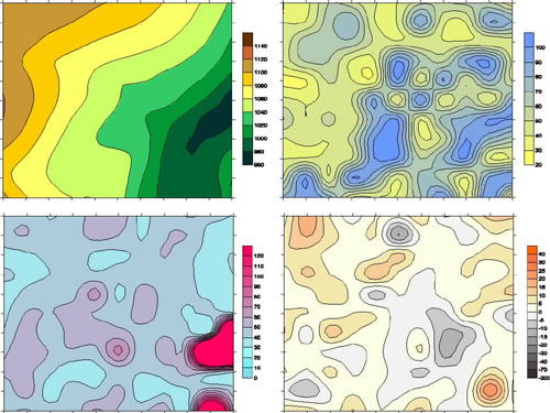
You never know what you'll find walking across the tundra... a beautiful view of the Brooks Range, a herd of musk oxen, or Javier probing a Grid (photo by Anna Klene). IV. Analysis: What we learned from this summers data. Don and Javier came to the University of Delaware in November to assist in data analysis. Records from each ARCSS grid for each year from 1995 to 1998 were examined and maps constructed of the deepest (mid-August) thaw each year, and of the four-year mean at each site. Then more maps were made of the yearly deviation from the mean at each site. The illustration below shows an example of the four-year mean active-layer thickness maps and 1998 deviation from the four-year mean maps for two sites, one from the coastal plain, and one from the foothills. Notice how smooth the two maps on the bottom left (Barrow) are in comparison to those on the bottom right (Happy Valley). Barrow
Happy Valley
Barrow (coastal plain). Top row: elevation (m), soil moisture (%); bottom row: four-year mean mid-August active-layer thickness 1995- 1998 (cm), differences between 1998 active-layer thickness and the four-year mean (cm, positive numbers indicate deeper thaw than mean). Happy Valley (foothills). Top row: elevation (m), soil moisture (%); bottom row: four-year mean mid-August active-layer thickness 1995- 1998 (cm), differences between 1998 active-layer thickness and the four-year mean (cm, positive numbers indicate deeper thaw than mean).
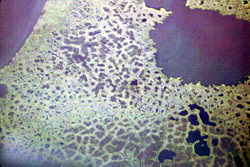
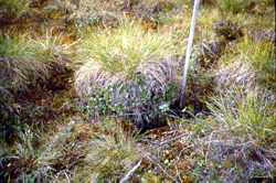
Above left: Aerial view of a typical section of the coastal plain: notice the polygonal patterns, formed by ice wedges under the ground. Water often forms small ponds in the depressed centers of the polygons. The two lakes in the photo are typical of the thousands occurring in the outermost coastal plain. Above right: A tussock in the foothills. This one is approximately 15 inches tall, which is fairly small. They make surface processes hard to estimate, and walking on them has been compared to walking on basketballs. The summer of 1998 was warm, contributing to a thicker overall active layer than had been observed the previous three years. As the two difference maps illustrate, however, a great deal of variation exists within each grid allowing some areas to be thinner than usual. Dry areas tended to thaw deeper than usual due to the hotter temperatures, while the usually wet areas exhibited different reactions depending on whether some water was still present at the surface this year, or if less water than usual was present within the soil matrix.
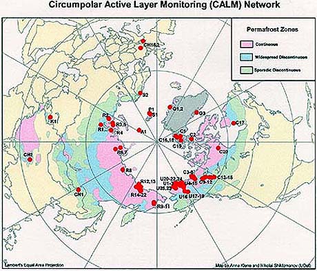
Click on the map to go to the CALM web site. Three regions of permafrost are shown: continuous, discontinuous and sporadic. Continuous permafrost can be interpreted as areas where permafrost is found everywhere beneath the ground at some depth. Discontinuous areas are regions where permafrost is very common, but not present everywhere. Sporadic areas indicate regions in which conditions are marginal for the formation or maintenance of permafrost and its existence is dependent on vegetation and soil characteristics. A longer data record is needed before quantitative
estimates of inter-annual variability are feasible, but we can conclude
from the four-year data that substantial differences do occur. As
part of a larger research effort, our data sets were incorporated into
the Circumpolar Active Layer Monitoring (CALM) Network database.
CALM is an international effort to coordinate data-collection procedures
and support long-term monitoring efforts. Climate change is expected
to impact active-layer thickness but few records exist over long enough
time periods to be able to determine how much change is "normal" interannual
variability and how much could be related to longer climatic trends.
Data collection over a larger area allows scientists to see if trends in
one area are similar to those founds in other parts of the world, which
may help us to understand regional differences in climate. This is
only possible through international cooperation.
May 2003
August 1998
July 1998
|


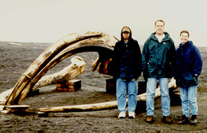 Javier,
Don and Anna check out a bowhead whale skull on the beach near Barrow on
a typical August day. (Photos courtesy of Don Rogers unless otherwise
noted).
Javier,
Don and Anna check out a bowhead whale skull on the beach near Barrow on
a typical August day. (Photos courtesy of Don Rogers unless otherwise
noted).
 The most practical means of measuring active-layer depth over large areas
is with a 1-cm diameter metal rod marked in 1-cm increments. This
rod is pushed vertically into the soil until it hits the ice-bonded permafrost
and the depth can be read. This is done twice at each of the 121
stakes on the ARCSS grids. At each flux site measurements are taken
along three transects at 5-m intervals for a total of 71 measurements.
Since some sites are a mile from the road in rough terrain, everyone gets
plenty of exercise.
The most practical means of measuring active-layer depth over large areas
is with a 1-cm diameter metal rod marked in 1-cm increments. This
rod is pushed vertically into the soil until it hits the ice-bonded permafrost
and the depth can be read. This is done twice at each of the 121
stakes on the ARCSS grids. At each flux site measurements are taken
along three transects at 5-m intervals for a total of 71 measurements.
Since some sites are a mile from the road in rough terrain, everyone gets
plenty of exercise.
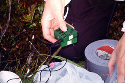 Temperatures are measured at each study site. The ARCSS grids have
data loggers recording air and soil temperatures year round. At each
Flux site air and nine soil-surface temperatures are monitored. These
match-book size data loggers are carefully packed in PVC pipe and plastic
bags to prevent foxes, lemmings, and other creatures from chewing on them,
and to prevent water damage. Each logger needed to have the data
downloaded, battery replaced, and be rewrapped for winter. To see
some results from research John Nevins parcticipated in last summer using
this temperature data click
Temperatures are measured at each study site. The ARCSS grids have
data loggers recording air and soil temperatures year round. At each
Flux site air and nine soil-surface temperatures are monitored. These
match-book size data loggers are carefully packed in PVC pipe and plastic
bags to prevent foxes, lemmings, and other creatures from chewing on them,
and to prevent water damage. Each logger needed to have the data
downloaded, battery replaced, and be rewrapped for winter. To see
some results from research John Nevins parcticipated in last summer using
this temperature data click 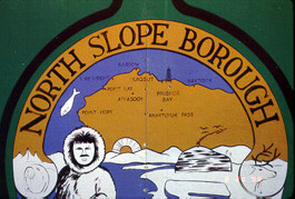 All
of our field activities took place within the North Slope Borough.
Alaskan boroughs are municipal governments in the way that counties are
the local government in many other states. Most of the people that
live in the borough are Inupiat, or native peoples. We stayed in
three different communities on our trip which
All
of our field activities took place within the North Slope Borough.
Alaskan boroughs are municipal governments in the way that counties are
the local government in many other states. Most of the people that
live in the borough are Inupiat, or native peoples. We stayed in
three different communities on our trip which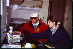 represent the many diverse activities that are happening in northern Alaska.
Our first home-away-from-home was Toolik Lake Field Station, operated by
the University of Alaska at Fairbanks for the National Science Foundation.
This camp accommodates up to 150 scientists and has been operating since
the mid-1970s. Facilities include a large dining hall, several dry
and one wet laboratories, and hard-sided trailers and tents for sleeping.
Recently, new labs, an e-mail connection and a shower have been added.
These comforts were much appreciated by our group. The next week
the group moved to
represent the many diverse activities that are happening in northern Alaska.
Our first home-away-from-home was Toolik Lake Field Station, operated by
the University of Alaska at Fairbanks for the National Science Foundation.
This camp accommodates up to 150 scientists and has been operating since
the mid-1970s. Facilities include a large dining hall, several dry
and one wet laboratories, and hard-sided trailers and tents for sleeping.
Recently, new labs, an e-mail connection and a shower have been added.
These comforts were much appreciated by our group. The next week
the group moved to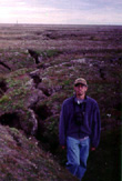 Deadhorse.
This community provides support functions for oil operations on the Prudhoe
Bay field, and most of the residents are temporary, working at the Post
Office, hardware store, general store, or for one of the airlines.
From Prudhoe, the group flew to Barrow, a community of 3500 residents.
It was a relief to see people of all ages going about their normal lives.
Learning about the native Inupiat culture added an extra dimension to the
last week.
Deadhorse.
This community provides support functions for oil operations on the Prudhoe
Bay field, and most of the residents are temporary, working at the Post
Office, hardware store, general store, or for one of the airlines.
From Prudhoe, the group flew to Barrow, a community of 3500 residents.
It was a relief to see people of all ages going about their normal lives.
Learning about the native Inupiat culture added an extra dimension to the
last week.
 These
differences confirmed our previous interpretations, based on statistical
analysis, about patterns of spatial variability in the coastal plain and
the foothills. The nearly flat coastal plain is dominated by ponding
in polygons, large elongated "thaw" lakes, and slightly higher (~1m) areas
in between. Differences in thaw depth are mainly due to how much
water is in the small, shallow ponds, if a point is close to a "thaw" lake
or in the intermediate areas. In contrast, the large rolling foothills
to the south are covered with stream networks and complex tussock, shrub
and moss vegetation. The micro-scale variation caused by differences
in the vegetation thickness, soil moisture content, and albedo of the landcover
allow more than 40-cm differences in active-layer thicknesses at points
just a few meters apart.
These
differences confirmed our previous interpretations, based on statistical
analysis, about patterns of spatial variability in the coastal plain and
the foothills. The nearly flat coastal plain is dominated by ponding
in polygons, large elongated "thaw" lakes, and slightly higher (~1m) areas
in between. Differences in thaw depth are mainly due to how much
water is in the small, shallow ponds, if a point is close to a "thaw" lake
or in the intermediate areas. In contrast, the large rolling foothills
to the south are covered with stream networks and complex tussock, shrub
and moss vegetation. The micro-scale variation caused by differences
in the vegetation thickness, soil moisture content, and albedo of the landcover
allow more than 40-cm differences in active-layer thicknesses at points
just a few meters apart.